
INTRODUCTION
The freshness of meat, which is a key factor that influences the purchasing decisions of consumers [1], depends on the temperature and humidity conditions under which the product is stored, and its level of microbial contamination. Fresh meat is rich in nutritional components, such as protein, fat, and minerals, and has high water activity, all factors of which provide a favorable environment for microbial growth. Under such conditions, various types of microorganisms can cause meat spoilage [2]. Therefore, addressing these microbial issues is important for food preservation. Strategies include chemical treatment, vacuum treatment, heat treatment, and drying, among which cold treatment by freezing and refrigeration is the most used method [3]. However, sudden temperature changes under poor cold-chain conditions in sanitary facilities or during product transport can cause microbial contamination. Given that microbial reactions can adversely affect the food product, the potential for metabolic activity by microorganisms should be identified in advance to ensure stable food preservation [4].
Currently, the determination of freshness is based on chemical-base indicators, such as pH, volatile basic nitrogen (VBN) content, and 2-thiobarbituric acid-reactive substance (TBARS) value, or microbial contamination indicators, such as the total viable count (TVC) and total aerobic bacterial (TAB) count [5–7]. DeGeer measured and compared various quality parameters (pH, moisture, and lipid contents, TBARS value, microbial contamination level, and shearing force) of heat-cooked meat to identify the optimal conditions for dry aging beef [8]. Cheng et al. tried hyperspectral imaging to accurately predict the total volatile basic nitrogen (TVB-N) content of grass carp fillets during frozen storage, demonstrating its potential for rapid and non-destructive fish freshness assessment [9]. Leonard et al. explored the effect of lupin flour on sausage attributes by preparing sausages with different contents and analyzing cooking loss, TBARS, texture profile, etc [10]. Lee proposed a system for monitoring changes in the quality of vacuum-packaged dry-aged beef during storage and predicting the shelf-life of the product based on its current state. The pH, CIE colors, TBARS value, VBN content, microbial contamination level, and sensory characteristics of the cooked meat were evaluated [11]. Chen proposed a novel approach for real-time prediction and analysis of food safety risks using the one-step kinetic integrated Wiener process (OS-WP). This approach achieved high accuracy in modeling microbial growth and provided valuable early warning information for risk management and decision-making [12]. Although these studies reported highly accurate results, the measurement of freshness using traditional analytical methods is difficult to apply in the field because the techniques can be time consuming and expensive [13].
To facilitate efficient food quality certification, vendors or evaluation agencies require highly reproducible and accurate technologies to rapidly identify the conditions of fresh and processed meats. One technology that can meet this need is near-infrared spectroscopy (NIRS), a non-destructive technique that offers the advantages of rapid measurement of a single sample and ease of data collection [14–16]. However, NIRS provides only one spectrum for a single round of data collection and yields no spatial information about the sample. Hyperspectral imaging (HSI) was developed to overcome the disadvantages of NIRS and has demonstrated the potential to provide both spatial and spectral information simultaneously [17]. As a non-destructive and contactless technique, HSI involves the integration of both spectral and imaging technologies for the examination of various components in samples. The system generates three-dimensional data in the form of a so-called hyperspectral data cube composed of a two-dimensional spatial image and a one-dimensional spectrum [18]. These data cubes can be used to analyze physical and geometrical characteristics (including morphology, color, and size) of an image, and the chemical composition of the sample can be predicted with an artificial intelligence model constructed using spectral information [19].
Various studies have employed hyperspectral imaging technology for non-destructive quality evaluation of livestock and seafood products. These studies have ranged from non-destructive analysis of omega-3 fatty acids in eggs to predicting fat content in pork and analyzing the frozen state of fish fillets and pork loins [20–22]. Kamruzzaman showed that hyperspectral imaging and multivariate analysis can be used to identify red meat species (pork, beef, lamb) with 98.67% accuracy, demonstrating the potential for rapid and objective meat authentication [23]. Wold developed a near-infrared (NIR) spectroscopy method for online and non-contact monitoring of core temperature in heat-treated fish cakes during industrial processing, achieving a root mean square error of prediction of 2.3°C [24]. Yang used HSI to predict the level of protein deterioration during pork drying, whereas Aheto et al. used the method for predicting the TBARS value of dry-cured pork [25,26]. Lohumi et al. applied analysis of variance (ANOVA), spectral similarity analysis, and HSI in the 400–1,000 nm range to develop a system for predicting and visualizing the intramuscular fat content in beef samples. Advances in HSI technology have also led to studies on portable hyperspectral devices [27].
Consumer behavior towards meat and meat products is exhibiting increasing complexity and less predictability. And environmental impact has become significant driver of consumer perception [28]. Obviously, there is great scientific value in precisely determining the parameters that determine meat quality in the lab, whether by chemical methods or by directly observing microbial growth. However, these traditional tests are sometimes time-consuming and procedurally complex [29], therefore, several types of spectral analysis methods were employed and showed some promising solutions. However, a single point spectrum may not adequately represent the condition of the entire meat sample, which remains a drawback [30]. Accordingly, the aim of the present study is to use various machine learning techniques to develop a high-quality predictive model that can match hyperspectral imaging data with TAB counts for beef stored under different temperature conditions. It is to achieve precise identification of the contamination state of meat by combining microbiological factors and hyperspectral data. As a result, the study provided clues to optically visualize the distribution of microbial contamination in beef that could not be obtained by previous destructive chemical methods.
MATERIALS AND METHODS
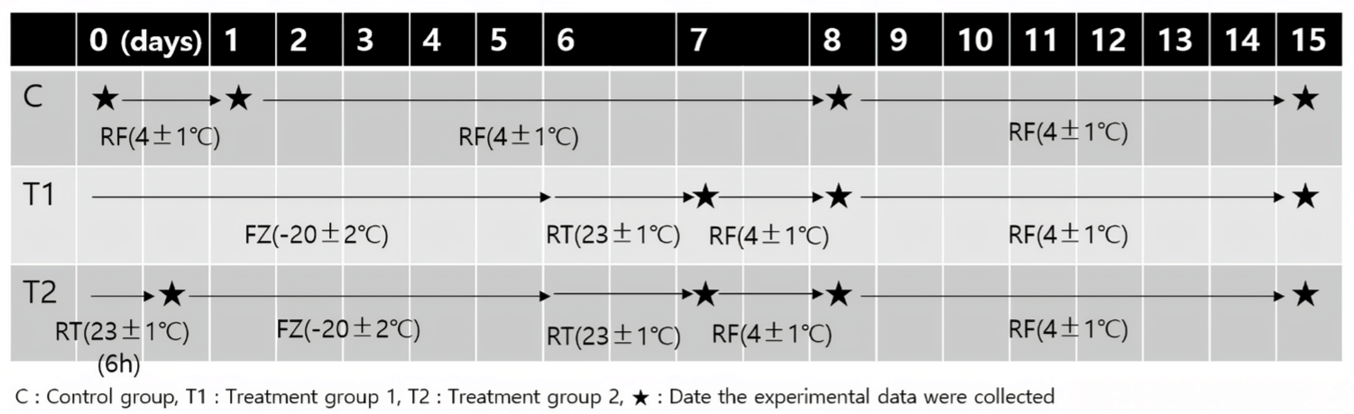
Experimental samples were obtained from the M. longissimus thoracis muscle chunks of three Korean Holstein cows. The average weight of the muscle chunks was 5.57 ± 0.61 kg. The beef chunks were purchased shortly after slaughter. Immediately following their acquisition, the three beef chunks were placed in a refrigeration box that was maintained at a temperature of 3 ± 1°C and transported to the laboratory. The meat samples were stored in the laboratory for 7 d at 4°C to achieve stabilization prior to the commencement of the experiment. After the stabilization period, the meat was removed from the vacuum package and the fascia and fat were excised. The resultant lean meat was cut along the direction of the myofiber into portions of approximately 250 g, which were then packed in shape to allow air flow. This was designated as the experimental start date. The experiment was conducted for 15 d and comprised the following three groups. The samples of control group were stored in a 4°C refrigerated environment throughout the experiment. Samples of Treatment group 1 were frozen at –20 ± 2°C for 6 d and thawed at 23 ± 1°C for 24 h to affect the microbial quality of the samples, and the rest of the period was refrigerated under the same conditions as the control group. And the last samples of treatment group 2 were initially left at 23°C for 6 h to induce microbial growth and the subsequent process is the same as treatment group 1. The experimental protocols are shown in Fig. 1.
The traditional plate count method was performed to obtain the reference of TAB count value. The measurement was performed in the following order, with some adjustments based on previous research [31–33]. First, 10 g of samples were immersed in 90 mL of 0.1% peptone water and homogenized with a mixer (BagMixer, Interscience) to properly disperse and dilute the microorganisms. 10-fold serial dilutions of the homogenate were prepared using sterilized peptone water. Then, 1 mL of the dilution was inoculated into liquefied agar medium melted at 45°C (plate count agar, Becton Dickinson), and the suspension was carefully shaken to mix the microorganisms evenly. The suspension was cultured in a 37°C incubator for 48 h, following which the number of resultant colonies was counted and expressed in units of Log CFU/g. The experiment was repeated three times.
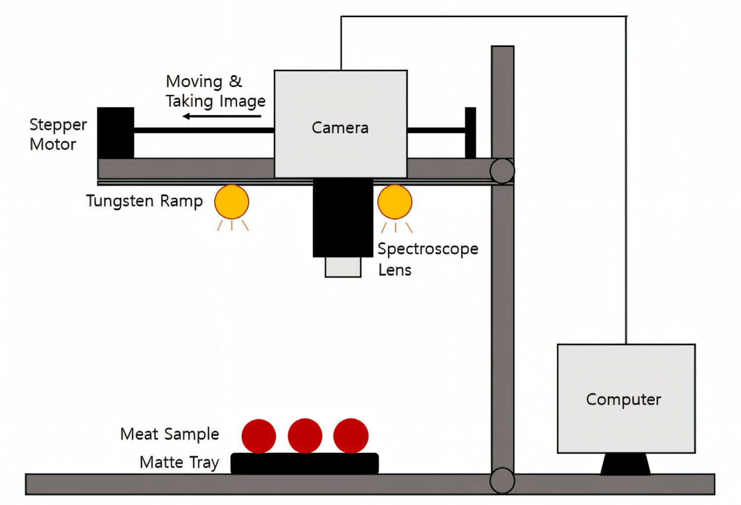
To acquire hyperspectral images, a darkroom environment was employed to block external light and an image acquisition system was installed inside. No special temperature control was installed in the darkroom. At that time, the room temperature was observed as 23°C–24°C. As shown in Fig. 2, the system consisted of a hyperspectral imaging camera (Pika L, Resonon) with an attached lens. The camera was mounted on a stepper motor to allow its movement along a line while taking images. Four tungsten halogen lamps were installed to secure a stable light source. A black matte dish was used as the sample background. A total of 99 beef samples were used. For each experiment, nine samples from the same group were photographed at the same time and subjected to microbiological analysis. To ensure the stability of the light source and obtain high-quality hyperspectral data, a 20 min stabilization period was implemented before data acquisition.
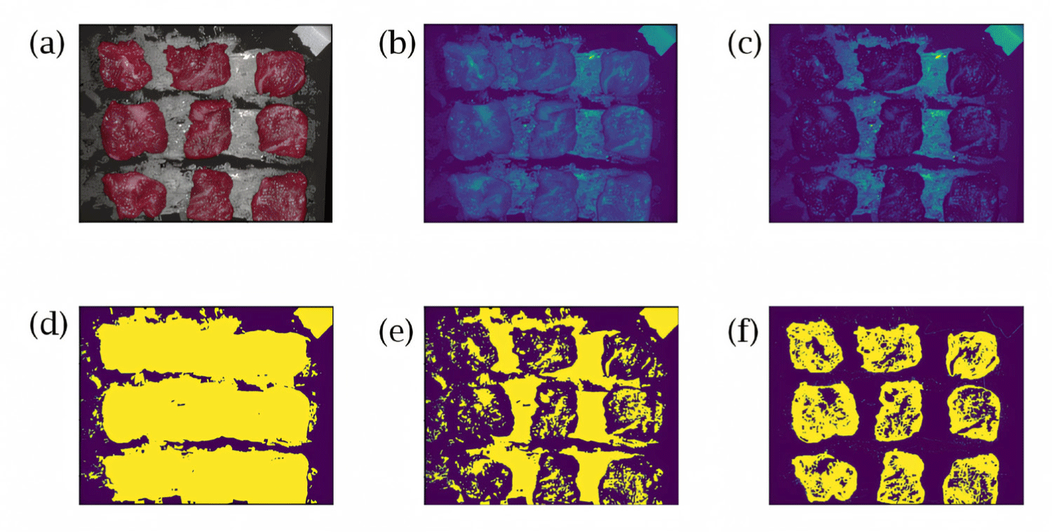
Next, the region of interest (ROI) was defined as the red meat region within the meat data, and spectrum of only this region was extracted for analysis. The processes for determining the area of red lean meat in the hyperspectral data cube are presented in Fig. 3. Fig. 3A was reconstructed using only the visible light region (400–700 nm), whereas Fig. 3B was extracted from spectral images in the 630–650 nm range as an average value corresponding to the red region. Fig. 3C is an extraction of only images having a wavelength of 540–560 nm, corresponding to the green area. By comparing Fig. 3B and 3C and generating their difference set, the red region can be extracted by selecting only the pixels that belong to the red region and neither to the black region nor to the white region. To achieve this, Fig. 3B and 3C were first converted into binary images, resulting in Fig. 3D and 3E, respectively. As the result, Fig. 3F shows the difference between the two binary images. Consequently, by selecting and extracting only the spectra from the activated region in Fig. 3F, the spectra of red meat can be exclusively obtained.
The extracted spectrum data for the area of red lean meat were used to develop TAB prediction model. And four machine learning methods were employed including partial least squares regression (PLSR), support vector machine (SVM), artificial neural network (ANN), and one-dimensional convolutional neural network (1D-CNN). Also, four preprocessing techniques such as multiplicative scatter correction (MSC), standard normal variate (SNV) transformation, Savitzky–Golay 1st-order filtering, and min–max normalization were used. In addition, models named ‘raw’ were developed and these models used raw spectrum which are not preprocessed. In this study, 80% of the experimental data was used as the training set, and the remaining 20% was used as the test set to verify the model’s performance. The randomly selected training set was 10-fold cross-validated to validate performance and develop optimal models.
PLSR is known as a widely used technique for the quantitative analysis of spectra [34]. As a method that complements the shortcomings of principal component analysis, PLSR is used mainly for component prediction in the measurement field. It performs the least squares method by compressing data down to several latent variables containing the most information in a data set, including both the input variable X and the output variable Y. To develop the PLSR model, one data set—including both the X matrix obtained from the spectral data and the Y vector obtained from the TAB counts—was first generated. Then, the number of components with the lowest root-mean-square error (RMSE) value was selected while changing the number of components from 1 to 40. The model was finally constructed using the number of components. Through this procedure, it can be seen that both the calibration and validation processes can be performed at once.
The SVM technique was originally developed for classification purposes, but it can be applied for support vector regression (SVR) problems through the use of a loss function. In this study, ε-insensitive loss function was used as following Equation (1):
where yk is the kth element of the y vector, and fk(x) is the value predicted by the model.
To develop the ANN model, a structure with an appropriate layer had to be designed. In the ANN, the connection structure between neurons, such as the number of hidden layers and the number of nodes of each layer, is collectively referred to as a topology, the optimal determination of which generally requires a large number of trial-and-error runs [35]. In this study, performance was tested by varying the number of hidden layers and the number of nodes in the model. The hidden layers were either one or two, and the number of nodes in each layer started at 25 and increased by one to 35. The optimal topology was found to be two hidden layers with 32 nodes each. The rectified linear unit (ReLU) was used as the hidden layer activation function, and adaptive moment estimation was used as the optimizer in the compilation process.
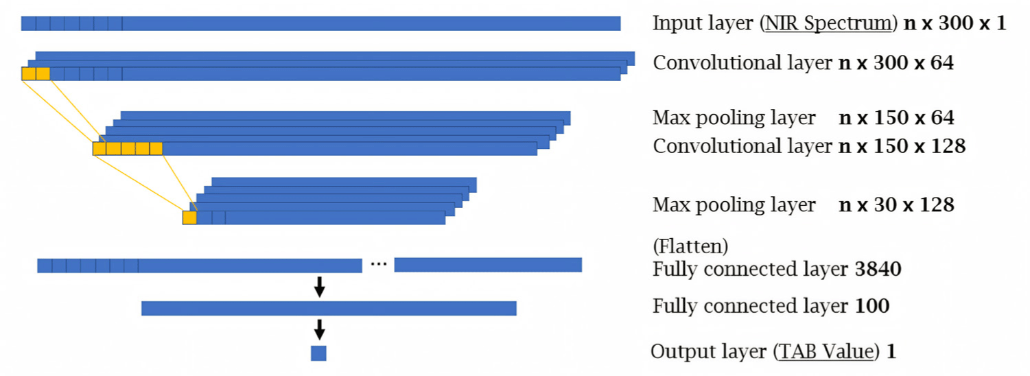
A CNN-based model, which is a class of ANN, is the most widely used architecture in deep learning approaches. Of the various CNN techniques, 1D-CNN was used in our study because the extracted spectrum was one-dimensional signal. Generally, the structure of a CNN-based model consists of an input layer, multiple hidden layers (convolutional layers, pooling layers, fully connected layers), and an output layer [36]. A structure of 1D-CNN based model also comprises a convolutional layer and a 1D filter suitable for spectral data. As was carried out for the ANN, the layer structure for the 1D-CNN was determined through trial-and-error repetitions, and the one with the highest performance was selected. Additionally, a dense layer consisting of 100 nodes was added before the result was reached. The ReLU function was used for all hidden layers. Fig. 4 shows the structure of the 1D-CNN used in this study. Since the models were created using four different techniques, evaluation indicators were needed for the comparison of their performances. This was achieved through three commonly used indicators for the evaluation of predictive model: R2, mean absolute error (MAE), and RMSE, calculated using Equatios (2), (3), and (4), respectively:
where n is the total number of data points, Ai is the actual output values, Pi is the predicted output values, and A- is average.
To ensure the generalizability of the developed model, a rigorous verification process was implemented. While the training and test sets were strictly separated during model development, both used samples from the same carcass. This potential limitation in variability prompted an additional verification step. At a different time, completely different beef samples were purchased and stored under identical conditions to those used for model development. All procedures used for the training and test sets were meticulously replicated with these new samples to create a dedicated verification set. This verification set was then applied to the previously developed models to assess their versatility.
RESULTS AND DISCUSSION
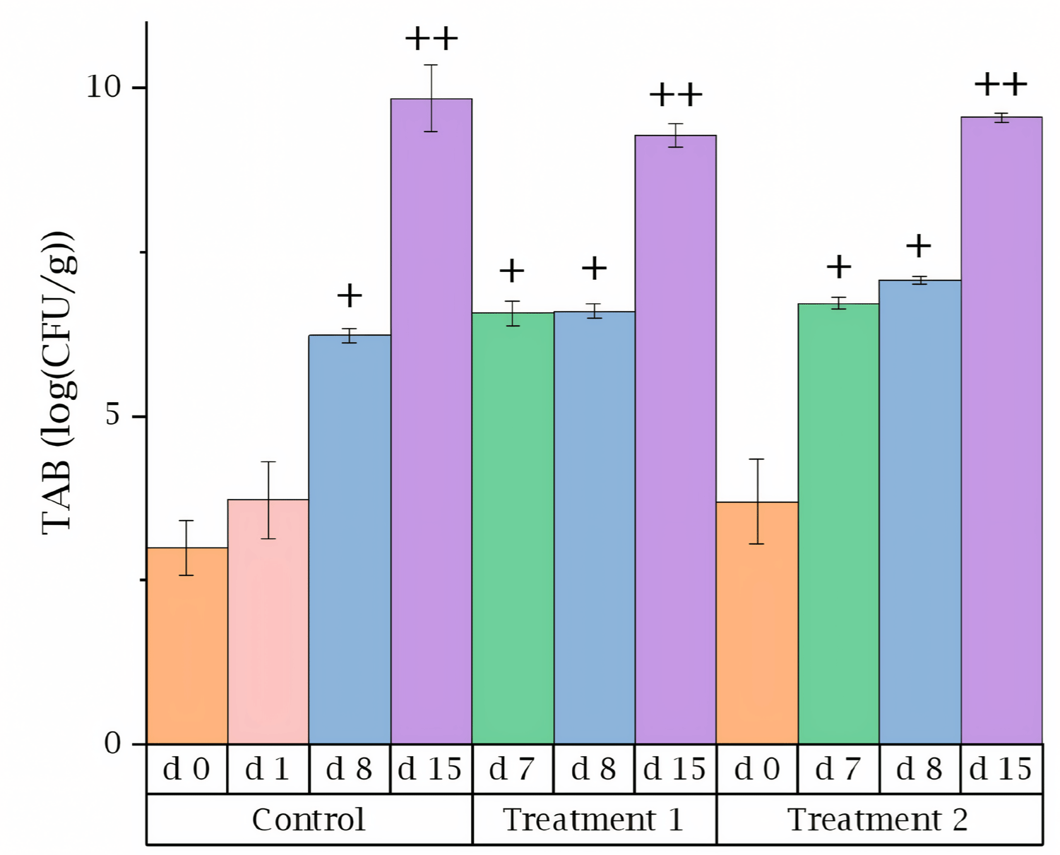
Fig. 5 shows the TAB values for different treatments of the beef samples. Similar to the results reported by other research, the TAB increased by approximately 3 folds with each passing week [37]. And no specific packaging or air conditioning treatments were applied to the samples, resulting in higher microbial counts compared to previous study [38]. Statistical differences among the results were evaluated using Scheffe’s post hoc test, with a significance level set at 5%. For this analysis, SPSS 26.0 statistical software package (IBM) was utilized. As anticipated, the five experimental dates clustered into three distinct groups based on their proximity. Furthermore, the analysis revealed that storage duration had a more pronounced effect on the proliferation of TAB.
A total of 5,285 spectra were extracted from the hyperspectral images of red meat area. The entire data set (n = 5,285) was then divided into a training set (n = 4,228) and a test set (n = 1,057). Table 1 shows the performance of the PLSR models in predicting TAB for different preprocessing methods. All models developed using the five data types achieved a coefficient of determination (R2) of 0.8 or higher, indicating successful training without significant issues. Evaluation on the five test data subsets likewise resulted in R2 values of 0.8 or greater. If the R2 values of the training and test sets were significantly different, it would suggest overfitting [39], but since this is not the case, it was determined that overfitting did not occur during the modelling process. The number of components in the PLSR models was in the range of 19–23.
The performance of the SVM, ANN, and 1D-CNN models is shown in Table 2. These models consistently outperformed the PLSR model in terms of prediction accuracy. When evaluated on the training set, almost all preprocessed data types achieved R2 values of 0.9 or higher, except 1D-CNN with some preprocessing methods. When testing SVM models, using data preprocessed by MSC achieved the best performance, with an R2 value of 0.9617 and an RMSE of 0.4659. And this result suggests that data preprocessing methods with scatter correction, such as MSC and SNV, are advantageous compared to other techniques. This finding is consistent with the SVM’s reliance on hyperplanes for class separation, as outlier removal through scatter correction can contribute to improved model performance.
As presented in Table 2, the predictive performance of the ANN model was superior to that of the other models. The training set yielded R2 values of 0.99 or higher, whereas the test set yielded R2 values of 0.97 or higher, which indicated a fit of the model with the experiment data. The best performance during test was exhibited by the ANN model constructed using min–max normalization data, which yielded an R2 value of 0.9926 and RMSE value of 0.2114. This is comparable to or slightly better than previous study [16]. The 1D-CNN models were the only ones that showed significant deviations in performance according to the data preprocessing technique used. Since the 1D-CNN does not follow the basic structure of a CNN that extracts morphological characteristics, the development of a segmental structure through the extraction of only the red meat region from the original hyperspectral data cube did not affect the interpretation of the results.
Fig. 6 presents the best test result for four models. Among these models, the ANN model with min-max normalization achieved the superior predictive performance. As can be observed in Fig. 6A and 6B, the PLSR and SVM based models exhibited lower performance compared to ANN and 1D-CNN based models shown in Fig. 6C and 6D, respectively. This is well illustrated by the wider distribution of predictions for samples sharing the same reference value in Fig. 6A and 6B. Consequently, it is reasonable to posit that prediction using neural network architecture offers a more viable modeling approach.
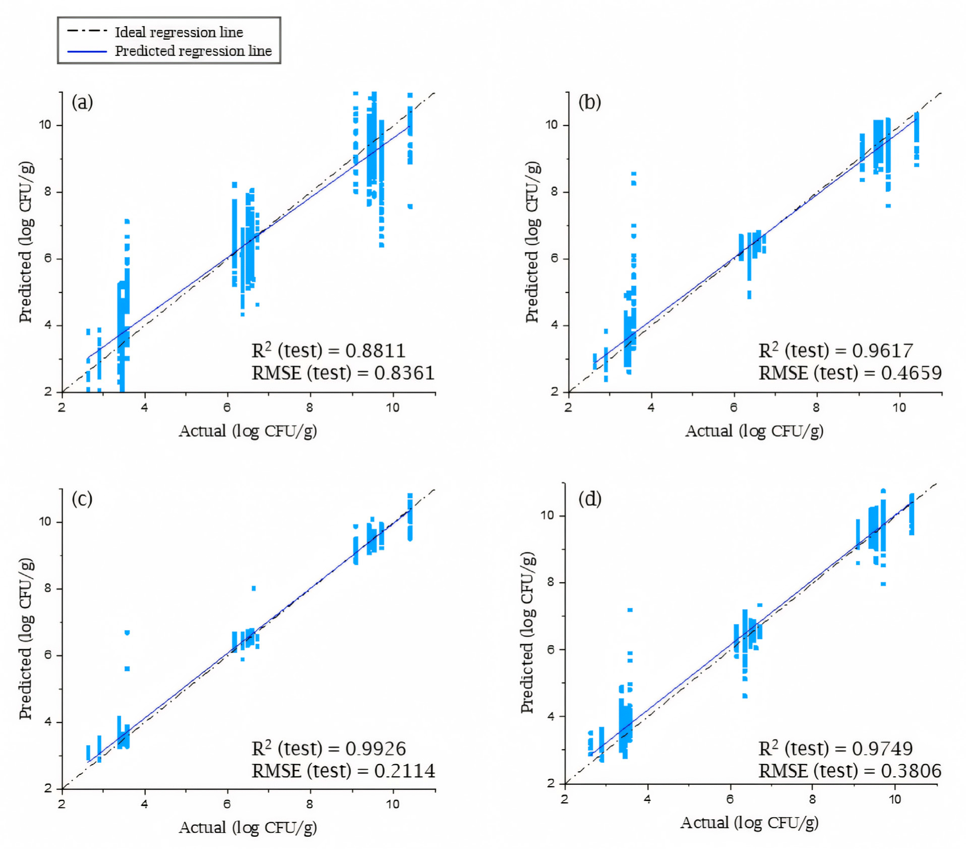
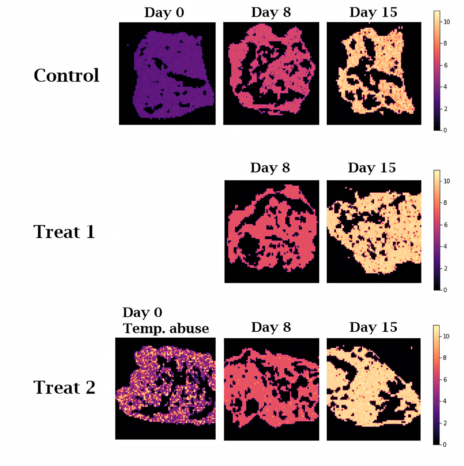
Fig. 7 shows the chemical map of predicted TAB count generated by inputting the hyperspectral data extracted from the red meat into the ANN model, which was identified to have the best predictive performance. Since only the spectral data extracted from the red meat area were used, all regions other than the red meat appeared as black spaces. This method allowed for direct visual observation of the differences in microbial quality of beef samples from each experimental group. Compared to previous studies [40], we demonstrate that the time-dependent microbial quality changes of beef samples were more clearly discernible due to the enhanced resolution and contrast provided by our study. The control group samples that were kept in refrigerated storage showed a generally uniform color distribution. The result suggests that an inappropriate storage method could cause deterioration of the meat quality that may be undetectable by visual inspection.
As a final step, additional experiments were conducted to verify the practical performance of the TAB prediction models which were presented in Tables 1 and 2. For this purpose, the TAB prediction performance of developed models was re-evaluated on a completely separate new beef samples from the beef samples used in the development of TAB prediction models. Table 3 shows the test performance of the best models for predicting TAB during the first model development process and the final verification step. As a result of verification test, it was observed that the R2 of the PLSR model decreased by 42.78% compared to the test results specified in Table 1. However, the R2 values of the other three models, SVR, ANN, and 1D-CNN based prediction models, were confirmed to be 0.7988, 0.8593, and 0.8479, respectively. These results are 16.94%, 13.43%, and 12.76% lower than the R2 values of the SVR, ANN, and 1D-CNN based prediction models shown in Table 2, respectively.
Although it was confirmed that the TAB prediction performance for completely new beef samples was reduced, the RMSE of the ANN and 1D-CNN based models acquired during verification test were 0.6947 and 0.681, respectively. These RMSE results can be analyzed as having a prediction error of about 7%, considering that the TAB destructively measured in actual beef samples were distributed in the range of 2.5 to 10. Through the verification test results, it was also observed that models based on artificial neural network methods such as ANN and 1D-CNN show better prediction performance than other machine learning-based models. Also, these results show the same trend as the model evaluation results shown in Table 2. If learning data for more diverse beef samples is acquired and additional, periodic learning processes are performed, the performance of machine learning models that can predict specific ingredients can be expected to improve to a certain level. Although this study cannot be said to have developed a sufficiently satisfactory prediction model that can be applied to all beef samples, it confirmed the possibility of predicting the TAB of beef non-destructively and non-invasively using machine learning methods and hyperspectral imaging technique. Further empirical research applying the methods and models presented in this study could lead to the development of commercially viable beef quality evaluation technology applicable in real-life settings. Accurate quality prediction helps livestock breeders develop and apply better husbandry practices, which ultimately leads to higher quality beef production. These technologies also enable faster response to consumer demand, enabling product development to meet market trends. Collaboration between industry and academia will play an important role in integrating these advanced technologies into existing quality management systems.
CONCLUSIONS
In this study, models for the non-destructive prediction of TAB in beef samples using NIR hyperspectral data were developed. Beef samples were exposed to various temperature conditions for 15 d to induce microbial growth and changes in meat freshness. For each meat sample, spectral data were obtained using a hyperspectral imaging system, and the TAB values were evaluated using the conventional plate count method to derive the reference counts for microbial contamination levels. In total, 5,285 spectra were extracted for the raw spectrum data and divided into a training set (80%) and a test set (20%). Then, models were developed using the PLSR, SVR, ANN, and 1D-CNN techniques. The predictive performance of each model was evaluated using the performance indicators R2, MAE, and RMSE. The ANN model was found to have the best predictive performance when the data was preprocessed using the min-max normalization method. In addition, even in a verification experiment performed with completely different beef samples at a separate time, the ANN based TAB prediction models showed somehow acceptable performance (R2: 0.85).
Recently, machine learning or deep learning-based ANN, CNN techniques have shown good performance in various fields. This study also successfully demonstrated the potential of ANN and 1D-CNN models for predicting TAB in beef using NIR hyperspectral data. These results are consistent with the growing body of research demonstrating the effectiveness of deep learning architectures in various analytical tasks. In our study, while both 1D-CNN and ANN models achieved high predictive performance, the ANN structure consistently outperformed for all data preprocessing methods. Interestingly, 1D-CNN performance showed greater sensitivity to preprocessing techniques, suggesting the potential for further optimization in this area.
In our study, there were some difficulties or limitations associated with the experiment and data acquisition. The number of sample groups was set to only three, and the observed microbial values were grouped by experimental day, resulting in a less diverse microbial population compared to real-world situations. Also, the experimental period was considered insufficient to represent all actual situations in the field. These experimental conditions have limitations in securing the diversity that can occur in actual distribution situations. To improve the generalizability of the models, future research should include data with a wider range of TAB that reflects the natural variability of microbial quality in beef. In addition, exploring the integration of other relevant data sources, such as temperature or storage conditions, alongside NIR spectral data could potentially refine model accuracy. Nonetheless, the approaches suggested in this study have the potential to provide more feasible and efficient tools for non-destructive microbial quality assessment in the meat industry.